What Does the Future Buy?
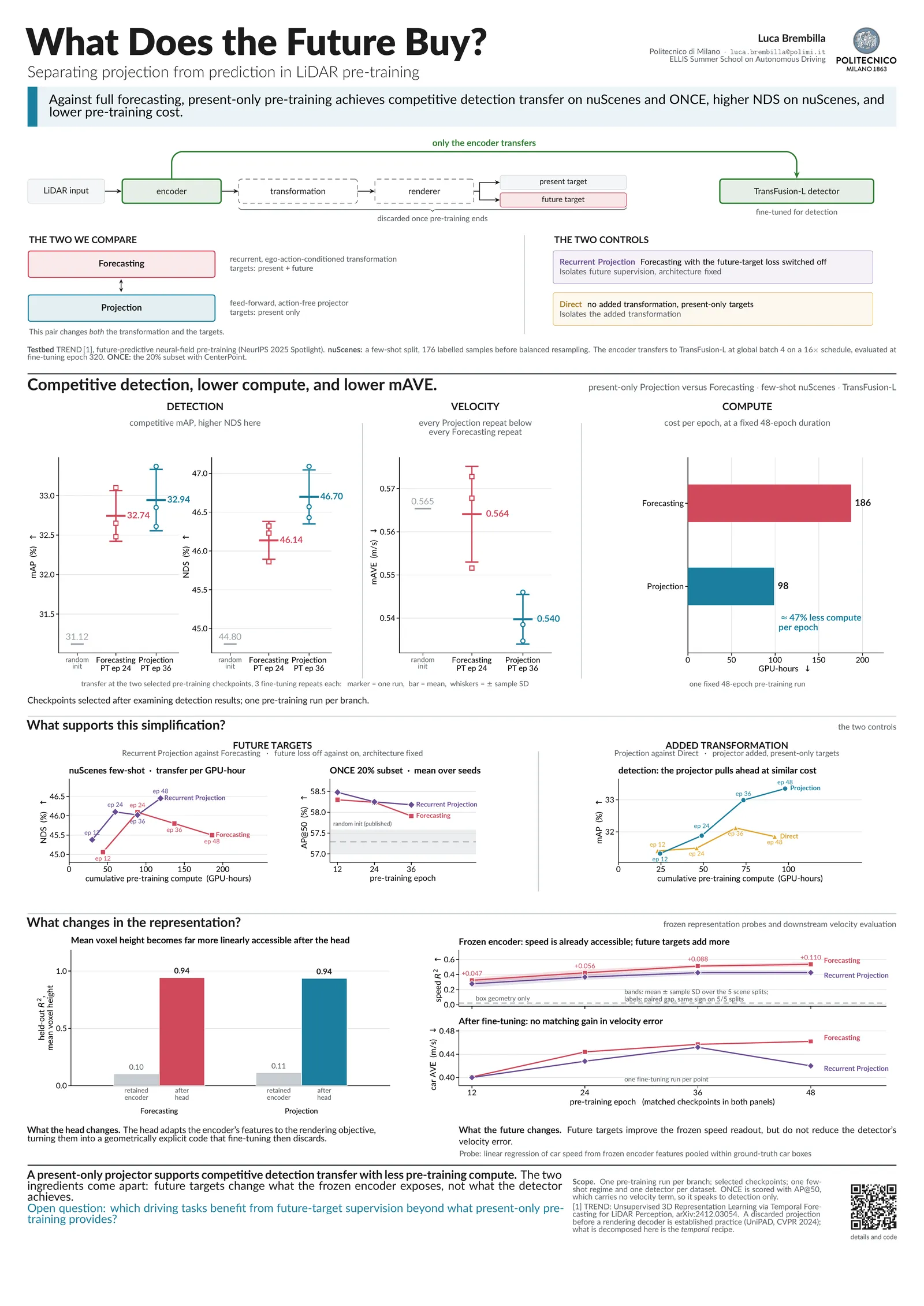
Future-predictive LiDAR pre-training combines a learned transformation with supervision from future scans. We separate the two. In the few-shot settings tested here, a present-only projector transfers competitively while using roughly half the pre-training compute per epoch; future targets make speed more accessible in frozen features without improving the detector's velocity error.
Forecasting changes two things
TREND pre-trains a LiDAR encoder by rendering the present scan and a future one, conditioned on the ego vehicle’s motion. This changes two ingredients together: it inserts a learned recurrent transformation between the encoder and renderer, and it adds future targets to the loss.
Only the encoder reaches the downstream detector. The transformation and renderer are discarded after pre-training. To find which ingredient supports transfer, we vary them one at a time over a shared scaffold:
- Direct: no added transformation, present targets only.
- Projection: an action-free feed-forward projector, present targets only.
- Recurrent Projection: the recurrent, action-conditioned transformation, with the future-target loss switched off.
- Forecasting: the same recurrent architecture, with present and future targets.
Two secondary controls test the role of the present anchor and the projector’s internal width. Together, the branches separate the effect of the added transformation from the effect of learning from future scans.
The practical result
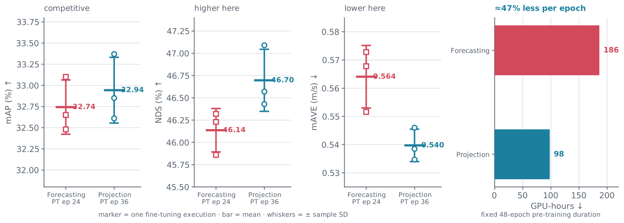
Projection and Forecasting are separated by only 0.20 mAP at the selected checkpoints, inside the observed fine-tuning variation. Projection has higher observed NDS and lower mAVE in all three fine-tuning executions, while its present-only objective requires about 47% less compute per pre-training epoch.
- +0.20mAP for Projection32.94 against 32.74
- +0.56NDS for Projection46.70 against 46.14
- ≈47%less compute per epoch98 against 186 GPU-hours over 48 epochs
The useful conclusion is a trade-off rather than a universal ranking: in this setting, the present-only projector retains competitive detection transfer at substantially lower pre-training cost.
The controls point in the same direction
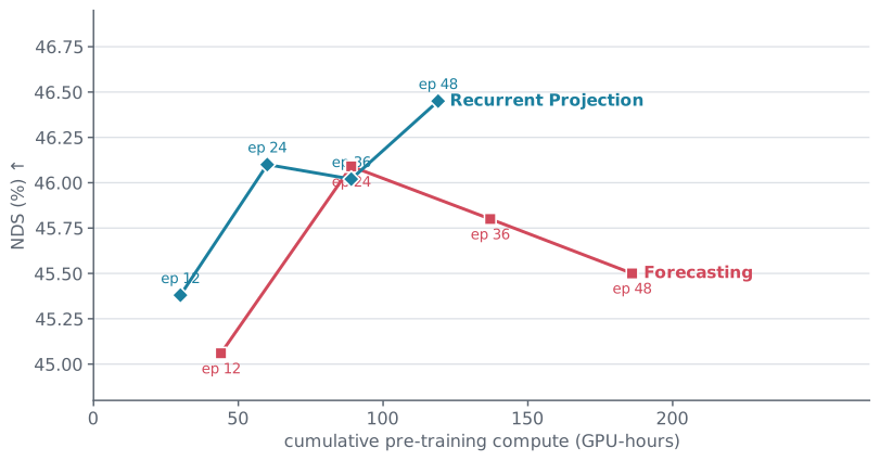
Holding the recurrent architecture fixed isolates future supervision. Across four matched pre-training checkpoints, switching off the future-target loss gives no consistent detection penalty and reaches comparable NDS with less compute.
ONCE provides a second detector and dataset. With three true fine-tuning seeds per cell, Forecasting, Recurrent Projection and the action-free Projection arm remain inside broadly overlapping spreads at both fully replicated checkpoints.
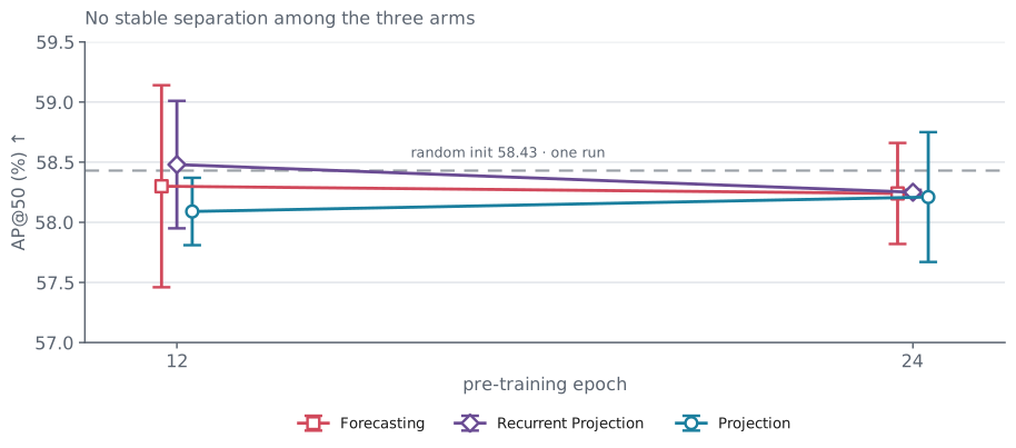
The original 59.26 Forecasting result at epoch 12 was the high realization of its cell; its three-seed mean is 58.30 ± 0.84. At epoch 24, the three means are 58.24, 58.25 and 58.21. ONCE therefore supports the relative conclusion—future targets and recurrence do not produce a stable advantage here—while the single scratch run does not support a precise absolute pre-training gain.
The transformation control is also directional on nuScenes. In the original executions, Projection exceeds Direct by 1.25 and 1.50 mAP at pre-training epochs 36 and 48, with the same direction in NDS. This is evidence that the discarded interface matters, although one pre-training trajectory per arm limits the precision of that comparison.
The discarded head formats the representation
What does the added transformation do? A frozen-checkpoint probe reads mean voxel height before and after it.
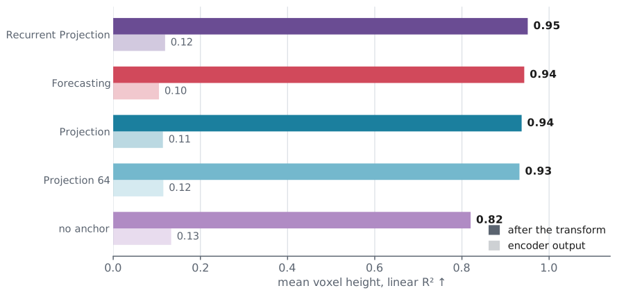
Mean height is only weakly linearly accessible at the encoder output, around 0.11 R², and becomes almost explicit after the head, around 0.94. The same effect appears with the action-free projector, the recurrent transformation and the half-width projector. This supports a simple interpretation: the discarded head formats abstract encoder features into a geometric, render-ready code. The probe characterizes the interface; by itself it does not establish why the retained encoder transfers better.
Future targets change what the encoder exposes
The second probe looks inside the part that survives. It pools frozen encoder features inside ground-truth car boxes and fits a linear speed readout on held-out scenes.
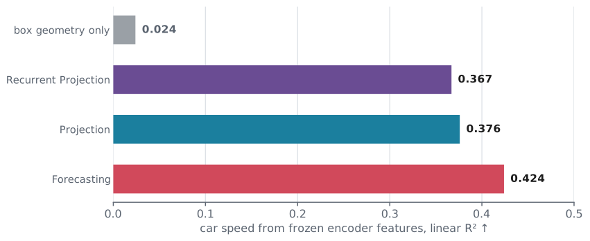
Speed is already accessible without future supervision: Recurrent Projection reaches 0.367 R² and Projection 0.376. Forecasting increases the readout to 0.424, with a positive paired difference on all five shared splits. Future supervision therefore reaches the retained encoder; it is not simply confined to the discarded prediction machinery.
That extra accessibility grows with the amount of future-supervised pre-training, but it does not become lower downstream velocity error in the detector.
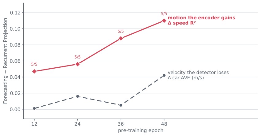
The clean result is a dissociation: future targets consistently improve this frozen linear readout within the measured trajectory, but the evaluated detector does not convert that improvement into better velocity estimates. At epoch 48, the largest readout difference coincides with the largest observed car-AVE cost; independent pre-training repeats would be needed to establish how general that endpoint is.
The two ingredients come apart. The added transformation supports detection transfer; future targets change what the frozen encoder exposes without improving the downstream velocity result observed here.
What this establishes—and what it does not
- One pre-training run per arm. The displayed repeats measure downstream fine-tuning or probe-split variation, not pre-training run-to-run variation.
- Selected checkpoints. The main result compares Forecasting at epoch 24 with Projection at epoch 36 after inspecting detection results. The matched trajectories provide the complementary control.
- Compute accounting. Forecasting’s cost is measured from training timestamps. The current-only costs are calibrated estimates for the intended objectives; the supplement records the full accounting.
- Probe scope. The motion result concerns linear accessibility for
vehicle.carin one few-shot regime. Five paired splits exclude split noise, not model-training variance.
These constraints make “competitive detection transfer” the supported claim. Higher NDS, lower mAVE and the speed-readout dissociation are observations in the evaluated setting, rather than estimates of a universal advantage.
The open question
Future supervision makes motion more accessible to a frozen linear readout, yet the detector does not spend that information here. Which driving tasks benefit from future supervision beyond what present-only pre-training provides? Motion segmentation and occupancy forecasting are natural places to look next.
The printed version
The argument is compressed onto one A0 sheet for the ELLIS Summer School on Autonomous Driving, September 2026.